You can skip through questions or sections; you are not required to answer the questions in sequence. The quiz will remember what questions you have answered, so you can go away from the quiz and return to it, keeping your place. Should you wish to begin again, and answer the questions a second time, simply press the Start Over message.
When the boxes into which you mark your answer are round, there is a single correct answer; however when the boxes are square, there is more than one correct answer. Click Submit answer when you have chosen your answer. You will receive messages about why your answer was correct or why your answer was not correct.
Comparison of plot sampling and distance sampling
Distance sampling is an extension of plot sampling, so there are some similarities between the two. These questions ask you to compare the two methods. The material under consideration comes from the first lecture in this chapter.
Extending plot sampling to distance sampling
These questions are from material found in this lecture. The topics here relate to the ideas of the covered region in distance sampling surveys and the important concept that distance sampling is a two-step process: the first step relies upon a model to make inference about animals not detected in the covered region and the second step relies upon the representativeness of the sampling design to make inference about animals not detected because the survey did not include the area where they reside.
Estimating probability of detection
You are introduced to several key functions defining detection functions in the chapter entitled Choosing a detection function. Please think about the consequences of the shape of detection functions upon your inference about population density as you answer these questions.
Estimating \(\hat{P}_a\)
Key functions
Provided the detection fitted to data at right, answer the following question.
.png)
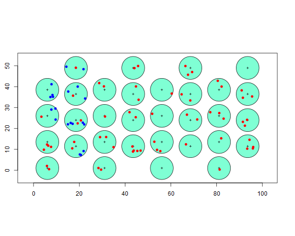
Calculation of abundance when information is available for some undetected animals
The diagram below shows the result of a point transect survey. The detected animals are indicated as red dots. For the western-most two rows of point transects, we are given information of not only the animals detected, but also the animals within the detection range, but undetected, are shown in blue. This is not the usual situation, but we include it so you can see how calculations are performed.
Ordinarily, we would fit a detection function to sighting data to produce our estimate of \(\hat{P_a}\), but here we employ some magic providing us with information about animals we do not detect on a few transects.
- The detection radius for each point is 5 units,
- there are 32 sampling points and
- size of rectangular study area is 5000 units
Calculations of density and abundance
To confirm computations made by program Distance, below are components from a line transect distance sampling survey and analysis needed to produce a density estimate. Use these components to answer the following questions, along with these formulas from slide 7 of lecture in Chapter 1.
\[ \hat{D} = \frac{n}{2wL \hat{P}_a} \hspace{2cm} \hat{N} = \frac{nA}{2wL \hat{P}_a} \]
| Area | CoveredArea | Effort | n | k | Encounter Rate |
|---|---|---|---|---|---|
| 630582 | 5270.514 | 1358.38 | 51 | 12 | 0.0375447 |
The truncation distance (\(w\)) for the survey was 1.94. In this situation, we have fitted a detection function to the sighting data and we have estimated the probability of detection of animals within the covered area \((\hat{P}_a)\) to be 0.5408.
Issues regarding detection functions and truncation
Detection functions should possess certain properties; think about those properties when answering the first question. Also discussed in this lecture is the subject of truncating data before fitting detection functions. Contemplate the reason behind truncation in your answer to that question.
The probability density function
The concept of a detection function is intuitive. However, the concept of a probability density function is more opaque. This set of questions gives you the opportunity to compare and contrast detection functions and probability density functions.